Free Recall Example
Nicholas Maxwell, Erin Buchanan
2021-12-06
Free_Recall.RmdLibraries and Data
Please see manuscript for a long description of the following data. We will load the example data, and you can use the ? with the dataset name to learn more about the data.
library(lrd)
#>
#> Attaching package: 'lrd'
#> The following object is masked from 'package:base':
#>
#>     kappa
data("wide_data")
head(wide_data)
#>   Sub.ID
#> 1      1
#> 2      2
#> 3      3
#> 4      4
#> 5      5
#> 6      6
#>                                                                                                Response
#> 1            basket, chair, clothes, flowrs, glasses, fan, windows, carpet, lamp, picture frame, remote
#> 2                                                                  windows, bed, books, shelf, pictures
#> 3 bacpack, chair, glasses, mirror, iphone, pillow, stereo, nightstand, computer, door, magazines, quilt
#> 4                                vase, blinds, computer, magazine, books, bed, blanket, carpet, dresser
#> 5                                                            bed, blankets, closet, windows, books, fan
#> 6                                     bed, blankets, dreser, nightstand, end table, stereo, flwrs, vase
#>   Disease.Condition
#> 1           healthy
#> 2           healthy
#> 3           healthy
#> 4              sick
#> 5              sick
#> 6              sick
#?wide_data

data("answer_key_free")
head(answer_key_free)
#>   Answer_Key
#> 1   backpack
#> 2     basket
#> 3        bed
#> 4    blanket
#> 5     blinds
#> 6      books
#?answer_key_free

library(ggplot2)
Data Restructuring
DF_long <- arrange_data(data = wide_data,
      responses = "Response",
      sep = ",",
      id = "Sub.ID")
head(DF_long)
#>   Sub.ID response position Disease.Condition
#> 1      1   basket        1           healthy
#> 2      1    chair        2           healthy
#> 3      1  clothes        3           healthy
#> 4      1   flowrs        4           healthy
#> 5      1  glasses        5           healthy
#> 6      1      fan        6           healthy
Data Cleanup
Scoring in lrd is case sensitive, so we will use tolower() to lower case all correct answers and participant answers.
Score the Data
You should define the following:
- data = dataframe of participant responses
- responses = column name of the participant answers
- key = column name of the answer key
- id = column name of the participant id number
- cutoff = the Levenshtein distance value you want to use for scoring (0 no changes exactly the same, higher numbers allow more variance in the word)
- flag = calculate z scores for outliers (TRUE/FALSE)
- group.by = column name(s) for grouping variables
free_output <- prop_correct_free(data = DF_long,
                                 responses = "response",
                                 key = answer_key_free$Answer_Key,
                                 id = "Sub.ID",
                                 cutoff = 1,
                                 flag = TRUE,
                                 group.by = "Disease.Condition")


str(free_output)
#> List of 3
#>  $ DF_Scored     :'data.frame':  51 obs. of  6 variables:
#>   ..$ Responses        : chr [1:51] "bacpack" "basket" "bed" "bed" ...
#>   ..$ Sub.ID           : num [1:51] 3 1 2 4 5 6 4 6 5 4 ...
#>   ..$ position         : num [1:51] 1 1 2 6 1 1 7 2 2 2 ...
#>   ..$ Disease.Condition: chr [1:51] "healthy" "healthy" "healthy" "sick" ...
#>   ..$ Answer           : chr [1:51] "backpack" "basket" "bed" "bed" ...
#>   ..$ Scored           : num [1:51] 1 1 1 1 1 1 1 1 1 1 ...
#>  $ DF_Participant:'data.frame':  6 obs. of  5 variables:
#>   ..$ Disease.Condition  : chr [1:6] "healthy" "healthy" "healthy" "sick" ...
#>   ..$ Sub.ID             : num [1:6] 1 2 3 4 5 6
#>   ..$ Proportion.Correct : num [1:6] 0.393 0.143 0.393 0.321 0.214 ...
#>   ..$ Z.Score.Group      : num [1:6] 0.577 -1.155 0.577 1.155 -0.577 ...
#>   ..$ Z.Score.Participant: num [1:6, 1] 1.082 -1.31 1.082 0.399 -0.626 ...
#>   .. ..- attr(*, "scaled:center")= num 0.28
#>   .. ..- attr(*, "scaled:scale")= num 0.105
#>  $ DF_Group      :'data.frame':  2 obs. of  4 variables:
#>   ..$ Disease.Condition: chr [1:2] "healthy" "sick"
#>   ..$ Mean             : num [1:2] 0.31 0.25
#>   ..$ SD               : num [1:2] 0.1443 0.0619
#>   ..$ N                : int [1:2] 3 3
Output
We can use DF_Scored to see the original dataframe with our new scored column - also to check if our answer key and participant answers matched up correctly! The DF_Participant can be used to view a participant level summary of the data. Last, if a grouping variable is used, we can use DF_Group to see that output.
#Overall
free_output$DF_Scored
#>        Responses Sub.ID position Disease.Condition        Answer Scored
#> 1        bacpack      3        1           healthy      backpack      1
#> 2         basket      1        1           healthy        basket      1
#> 3            bed      2        2           healthy           bed      1
#> 4            bed      4        6              sick           bed      1
#> 5            bed      5        1              sick           bed      1
#> 6            bed      6        1              sick           bed      1
#> 7        blanket      4        7              sick       blanket      1
#> 8       blankets      6        2              sick       blanket      1
#> 9       blankets      5        2              sick       blanket      1
#> 10        blinds      4        2              sick        blinds      1
#> 11         books      5        5              sick         books      1
#> 12         books      2        3           healthy         books      1
#> 13         books      4        5              sick         books      1
#> 14        carpet      1        8           healthy        carpet      1
#> 15        carpet      4        8              sick        carpet      1
#> 16         chair      1        2           healthy         chair      1
#> 17         chair      3        2           healthy         chair      1
#> 18        closet      5        3              sick        closet      1
#> 19       clothes      1        3           healthy       clothes      1
#> 20      computer      3        9           healthy      computer      1
#> 21      computer      4        3              sick      computer      1
#> 22          door      3       10           healthy          door      1
#> 23        dreser      6        3              sick       dresser      1
#> 24       dresser      4        9              sick       dresser      1
#> 25     end table      6        5              sick          <NA>      0
#> 26           fan      1        6           healthy           fan      1
#> 27           fan      5        6              sick           fan      1
#> 28        flowrs      1        4           healthy       flowers      1
#> 29         flwrs      6        7              sick          <NA>      0
#> 30       glasses      3        3           healthy       glasses      1
#> 31       glasses      1        5           healthy       glasses      1
#> 32        iphone      3        5           healthy          <NA>      0
#> 33          lamp      1        9           healthy          lamp      1
#> 34      magazine      4        4              sick     magazines      1
#> 35     magazines      3       11           healthy     magazines      1
#> 36        mirror      3        4           healthy        mirror      1
#> 37    nightstand      6        4              sick    nightstand      1
#> 38    nightstand      3        8           healthy    nightstand      1
#> 39 picture frame      1       10           healthy picture frame      1
#> 40      pictures      2        5           healthy          <NA>      0
#> 41        pillow      3        6           healthy        pillow      1
#> 42         quilt      3       12           healthy         quilt      1
#> 43        remote      1       11           healthy        remote      1
#> 44         shelf      2        4           healthy         shelf      1
#> 45        stereo      3        7           healthy        stereo      1
#> 46        stereo      6        6              sick        stereo      1
#> 47          vase      6        8              sick          vase      1
#> 48          vase      4        1              sick          vase      1
#> 49       windows      2        1           healthy       windows      1
#> 50       windows      1        7           healthy       windows      1
#> 51       windows      5        4              sick       windows      1

#Participant
free_output$DF_Participant
#>   Disease.Condition Sub.ID Proportion.Correct Z.Score.Group Z.Score.Participant
#> 1           healthy      1          0.3928571     0.5773503           1.0819232
#> 2           healthy      2          0.1428571    -1.1547005          -1.3096965
#> 3           healthy      3          0.3928571     0.5773503           1.0819232
#> 4              sick      4          0.3214286     1.1547005           0.3986033
#> 5              sick      5          0.2142857    -0.5773503          -0.6263766
#> 6              sick      6          0.2142857    -0.5773503          -0.6263766

#Group
free_output$DF_Group
#>   Disease.Condition      Mean         SD N
#> 1           healthy 0.3095238 0.14433757 3
#> 2              sick 0.2500000 0.06185896 3
Other Possible Calculations
Serial Position
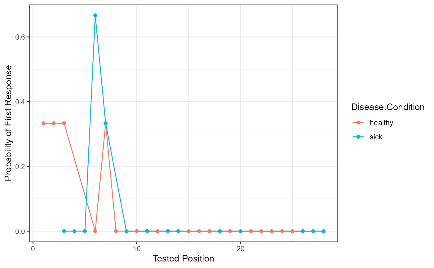
This function prepares the data for a serial position curve analysis or visualization. Please note, it assumes you are using the output from above, but any output with these columns would work fine. The arguments are roughly the same as the overall scoring function. We’ve also included some ggplot2 code as an example to help show how you might use our output for plotting. These graphs aren’t too exciting with a small example!
serial_output <- serial_position(data = free_output$DF_Scored,
                                 key = answer_key_free$Answer_Key,
                                 position = "position",
                                 scored = "Scored",
                                 answer = "Answer",
                                 group.by = "Disease.Condition")

head(serial_output)
#>   Disease.Condition Tested.Position Freq Proportion.Correct        SE
#> 1           healthy               1    1          0.3333333 0.2721655
#> 2           healthy               2    1          0.3333333 0.2721655
#> 3           healthy               3    1          0.3333333 0.2721655
#> 4              sick               3    0          0.0000000 0.0000000
#> 5              sick               4    0          0.0000000 0.0000000
#> 6              sick               5    0          0.0000000 0.0000000

ggplot(serial_output, aes(Tested.Position, Proportion.Correct, color = Disease.Condition)) +
  geom_line() +
  geom_point() +
  xlab("Tested Position") +
  ylab("Probability of First Response") +
theme_bw() 
Conditional Response Probability
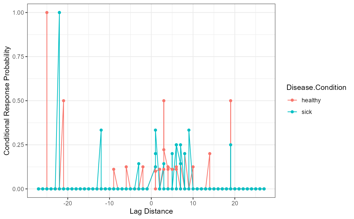
Conditional response probability is the likelihood of answers given the current answer set. Therefore, the column participant_lags represents the lag between the written and tested position (e.g., chair was listed second, which represents a lag of -6 from spot number 8 on the answer key list). The column Freq represents the frequency of the lags between listed and shown position, while the Possible.Freq column indicates the number of times that frequency could occur given each answer listed (e.g., given the current answer, a tally of the possible lags that could still occur). The CRP column calculates the conditional response probability, or the frequency column divided by the possible frequencies of lags.
crp_output <- crp(data = free_output$DF_Scored,
                  key = answer_key_free$Answer_Key,
                  position = "position",
                  scored = "Scored",
                  answer = "Answer",
                  id = "Sub.ID")

head(crp_output)
#>   Sub.ID participant_lags Freq Possible.Freq Disease.Condition CRP
#> 1      1              -27    0             0           healthy   0
#> 2      1              -26    0             0           healthy   0
#> 3      1              -25    0             0           healthy   0
#> 4      1              -24    0             0           healthy   0
#> 5      1              -23    0             0           healthy   0
#> 6      1              -22    0             0           healthy   0

crp_output$participant_lags <- as.numeric(as.character(crp_output$participant_lags))

ggplot(crp_output, aes(participant_lags, CRP, color = Disease.Condition)) +
  geom_line() +
  geom_point() +
  xlab("Lag Distance") +
  ylab("Conditional Response Probability") +
  theme_bw()
Probability of First Response
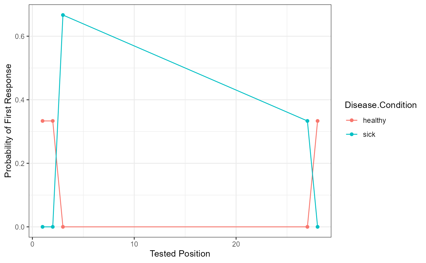
Participant answers are first filtered for their first response, and these are matched to the original order on the answer key list (Tested.Position). Then the frequency (Freq) of each of those answers is tallied and divided by the number of participants overall or by group if the group.by argument is included (pfr).
pfr_output <- pfr(data = free_output$DF_Scored,
                  key = answer_key_free$Answer_Key,
                  position = "position",
                  scored = "Scored",
                  answer = "Answer",
                  id = "Sub.ID",
                  group.by = "Disease.Condition")

head(pfr_output)
#>   Tested.Position Disease.Condition Freq       pfr
#> 1               1           healthy    1 0.3333333
#> 2               2           healthy    1 0.3333333
#> 3               3           healthy    0 0.0000000
#> 4              27           healthy    0 0.0000000
#> 5              28           healthy    1 0.3333333
#> 6               1              sick    0 0.0000000

pfr_output$Tested.Position <- as.numeric(as.character(pfr_output$Tested.Position))

ggplot(pfr_output, aes(Tested.Position, pfr, color = Disease.Condition)) +
  geom_line() +
  geom_point() +
  xlab("Tested Position") +
  ylab("Probability of First Response") +
  theme_bw()